
Signals and Sound · Course 1 · Lecture 1
Sound, signals and sampling
How does a sound become a list of numbers, and how do we get it back?
From a guitar string and a microphone to the sampling theorem, aliasing and the anti-aliasing filter, then the mathematics of aliasing and how the wave is rebuilt from its samples.
- A Level
- First year
- 25 min
- Eduqas A Level Electronics
- OCR A Level Physics B (Advancing Physics)
- Pearson Edexcel A level Music Technology
Checked by two AI reviewers against cited sources, 28 October 2026.Lecturer review pending.See the record
Plays from YouTube when you press play; nothing loads from YouTube before then. Captions in English (UK). Watch on YouTube
Read the full transcript · Workbook with notes, questions and answers (PDF)
At a glance
By the end, an A Level student can
- Read amplitude, period and frequency from a waveform and use .
- Explain sampling, and use and .
- State and apply the sampling theorem, , and the Nyquist frequency .
- Explain aliasing, and why the anti-aliasing low-pass filter comes first in a PCM transmitter.
A first-year student can also
- Show that and give identical samples, and calculate any alias frequency by folding.
- Explain why the anti-aliasing filter must be steep, and how oversampling eases it.
- Explain reconstruction: why, ideally, a filtered DAC output is the original band-limited wave, not a staircase.
Before this lecture: GCSE waves (frequency, wavelength, ). The first-year part uses the periodicity and symmetry of cosine; no calculus.
Key equations
- frequency and period
- sampling period
- the sampling theorem
- the Nyquist frequency
- any alias, k the whole number that makes it smallest
Part one · A Level
Notes: from a sound to a list of numbers
What a signal isin the video at 0:21
When a guitar string vibrates, it squashes and stretches the air beside it, and those squashes and stretches (compressions and rarefactions) travel outwards as a pressure wave at about 343 m/s in air at 20 °C. A microphone's diaphragm moves with the pressure, and the microphone turns that movement into a voltage: more pressure, higher voltage. That changing voltage is a signal, a quantity that changes over time and carries information.
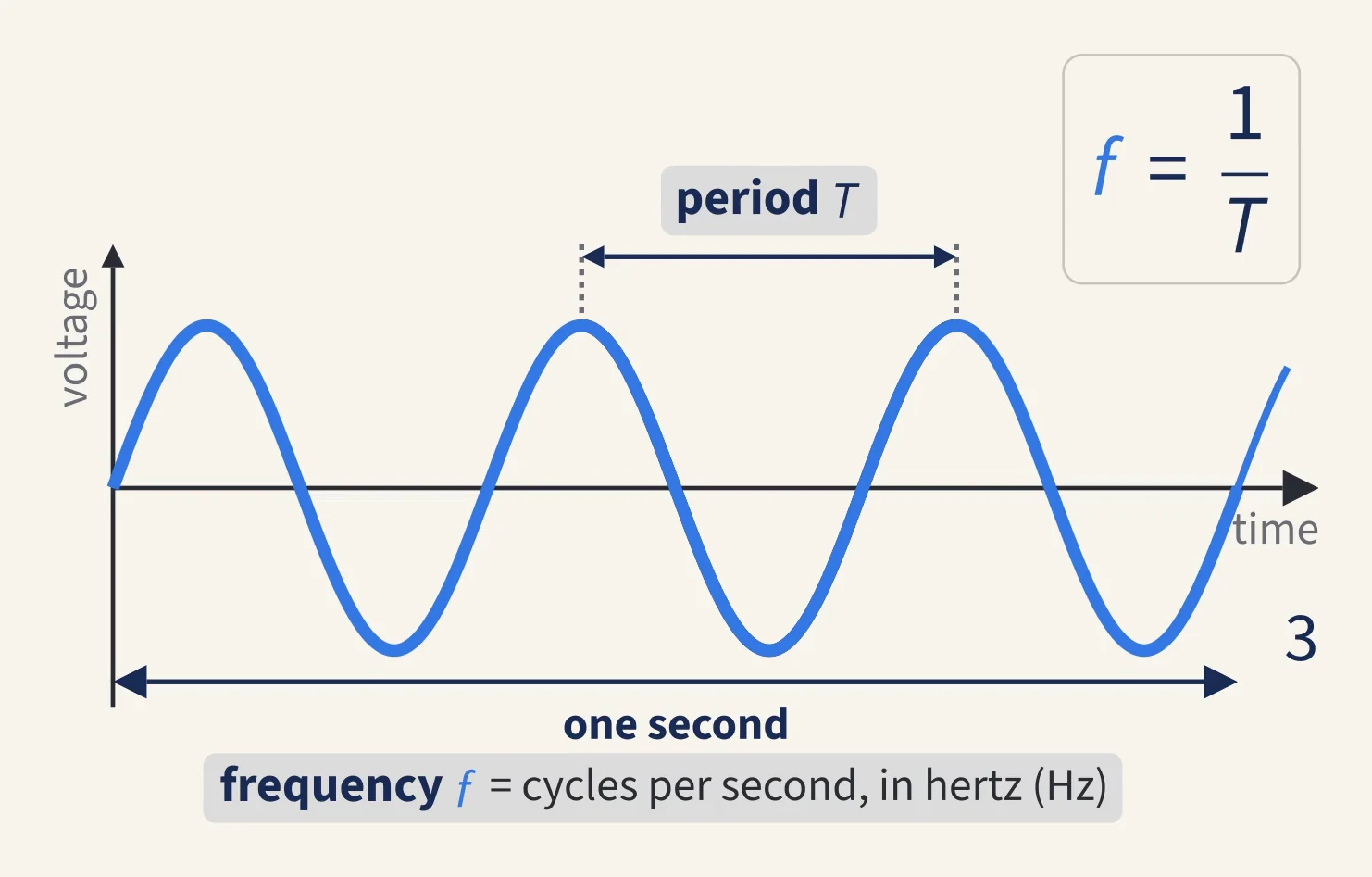
The simplest signal is a sine wave, the sound of a tuning fork. Its amplitude is the height from the middle line to a peak, and a bigger amplitude sounds louder. Its period is the time for one complete cycle, in seconds, and its frequency is the number of cycles each second, in hertz (Hz). They are two views of the same thing:
The A that orchestras tune to is 440 Hz, so its period is ms. Doubling a frequency raises a note by an octave; halving it lowers it by one.
Phase says where in its cycle a wave is at time zero, in degrees or radians. You cannot hear the phase of a single tone, but when signals are added together, phase decides whether they reinforce or cancel.
The range of hearingin the video at 3:11
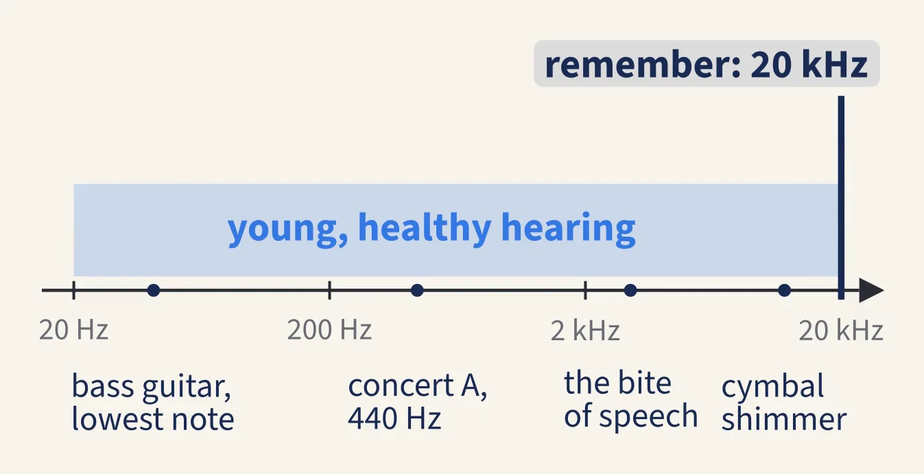
Young, healthy ears hear from about 20 Hz up to about 20 kHz. The top end falls with age, and many adults hear little above 15 or 16 kHz. That 20 kHz figure is what decides how fast audio has to be sampled.
Why go digital?in the video at 4:10
The microphone's voltage varies smoothly and continuously. It is analogue: a likeness, an analogue, of the pressure wave. Every time an analogue signal is copied, stored or sent, a little noise and distortion creep in, and in general they cannot be taken out again; copy a tape, then copy the copy, and by the fifth generation you can hear the hiss.
A digital signal is a list of numbers, and a number can be copied a million times without changing. Numbers can also be processed by a computer: filtered, mixed, compressed and sent round the world.
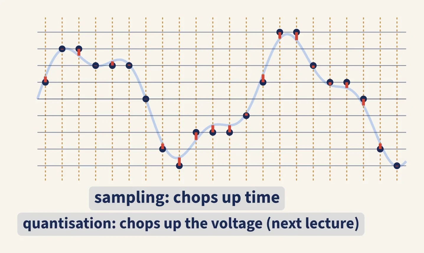
Turning a voltage into numbers takes two steps. Sampling measures it at regular moments in time, and is this lecture's subject. Quantisation rounds each measurement to one of a fixed set of levels, and is Lecture 2's. Sampling chops up time; quantisation chops up the voltage.
Samplingin the video at 5:33
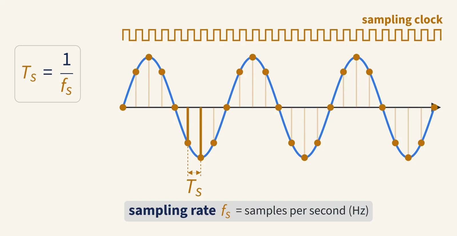
Imagine photographing the voltage at regular intervals and writing down each value. Each measurement is a sample. The number of samples taken each second is the sampling rate, or sampling frequency, , in hertz. The time between samples is the sampling period:
A CD samples at 44.1 kHz, 44 100 samples every second, so its samples are apart. Once a signal has been sampled the smooth wave is gone and only the dots remain. The question for the whole lecture is whether the wave can be got back from them.
On average, each cycle of a wave gets samples (any one cycle holds a whole number of them). At 44.1 kHz a 1 kHz tone gets 44.1 samples per cycle, and a 10 kHz tone gets 4.41: fewer, but still enough.
The sampling theoremin the video at 7:33
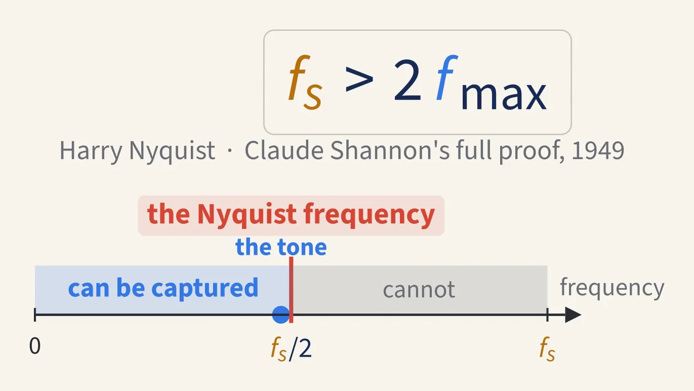
To capture a frequency you need more than two samples in each of its cycles. Put the other way round, the sampling rate must be more than twice the highest frequency in the signal:
This holds for signals that start at 0 Hz, such as audio. (A signal confined to a narrow band far above 0 Hz can be sampled more slowly, by a technique called bandpass sampling.)
This is the sampling theorem, often called the Nyquist theorem or the Nyquist–Shannon theorem. Its discovery was shared: E. T. Whittaker found the rebuilding formula in 1915, Harry Nyquist's 1928 telegraph work gave the factor of two, Vladimir Kotelnikov stated and proved it for communications in 1933, and Claude Shannon's 1949 paper, which gave the full proof for engineers and called the result common knowledge, made it famous. Half the sampling rate, , is the Nyquist frequency: the limit for a given sampling rate, since only frequencies below it can be captured.
Why more than two, and not exactly two? At exactly two samples per cycle the samples might land on the peaks, and the wave shows up, though its true size and phase still cannot be told. But they might equally land on the zero crossings, and then every sample is zero and the wave vanishes. Exactly two is not safe; just over two is enough.
Books differ in their words. Here, as in most audio work, the Nyquist frequency is . Oppenheim and Schafer instead call a signal's highest frequency its Nyquist frequency and twice that its Nyquist rate, and state the theorem with for a signal that has nothing at or above that frequency; Smith uses both names for .
Why a CD samples at 44.1 kHzin the video at 8:51
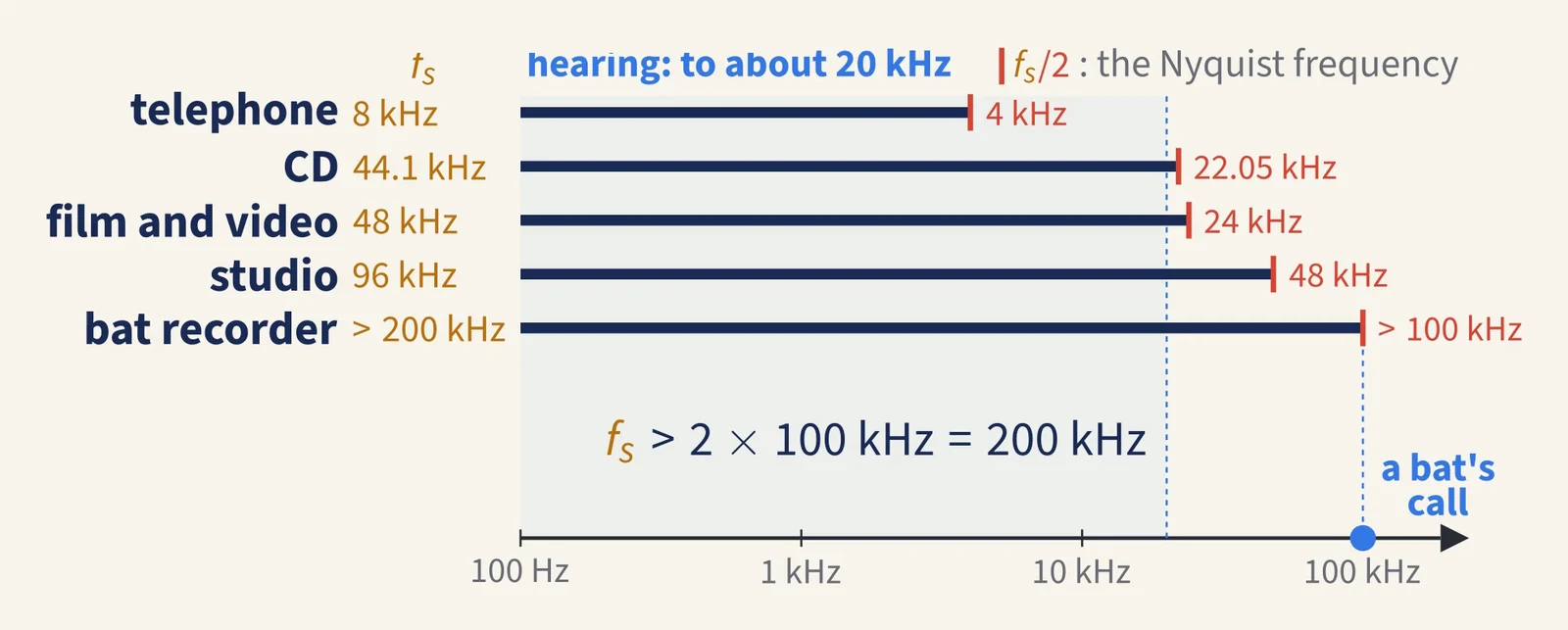
Hearing tops out at about 20 kHz, so audio needs a sampling rate above 40 kHz. A CD's 44.1 kHz gives a Nyquist frequency of 22.05 kHz, with a little room to spare, which the anti-aliasing filter needs (see below). The oddly precise number comes from history: the first digital recorders stored their samples on video tape, and 44 100 samples a second fitted the lines of a television picture exactly. In the European system that is 3 samples of each stereo channel on each of 294 usable lines, 50 fields (half-pictures) a second: . In the American system it is , at the 60 fields a second of black-and-white television; colour American television runs at 59.94, which gives 44 056.
Different jobs use different rates:
| Use | Sampling rate | Nyquist frequency |
|---|---|---|
| Traditional telephone | 8 kHz | 4 kHz |
| CD | 44.1 kHz | 22.05 kHz |
| Film and video | 48 kHz | 24 kHz |
| Studio recording | 96 kHz | 48 kHz |
A traditional telephone line carries about 300 Hz to 3.4 kHz, leaving room for the filter below its 4 kHz Nyquist frequency: enough to understand speech, but music loses its sparkle. Newer wideband ("HD voice") calls carry up to 7 kHz. Studios record at higher rates for more room while they work.
Aliasingin the video at 10:50
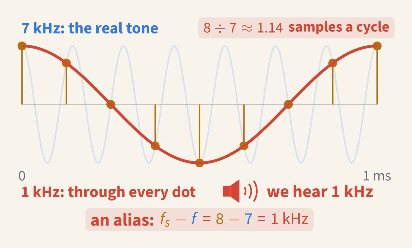
Break the rule and something strange happens. A film camera samples the world, usually 24 times a second. When a wheel's spoke moves almost a full spoke-spacing between one frame and the next, the camera cannot tell that it went nearly all the way forwards; the nearest match is a small step backwards. So a fast wheel seems to turn slowly backwards.
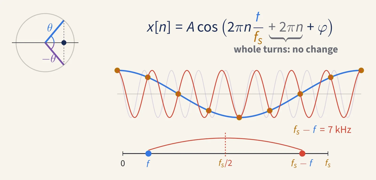
Sound does exactly the same. Sample a 7 kHz tone at 8 kHz, far fewer than two samples per cycle, and a gentle 1 kHz wave passes through every one of the samples. From the samples alone there is no way to tell which wave was there, and playing them back gives the 1 kHz tone. This impostor frequency is an alias, and the effect is aliasing.
A tone rising steadily past the Nyquist frequency is heard to turn round and fall, even though the real tone keeps rising. Everything above the Nyquist frequency folds back down, like a reflection in a mirror at ; above the folding repeats, as the first-year part shows.
The anti-aliasing filterin the video at 12:54
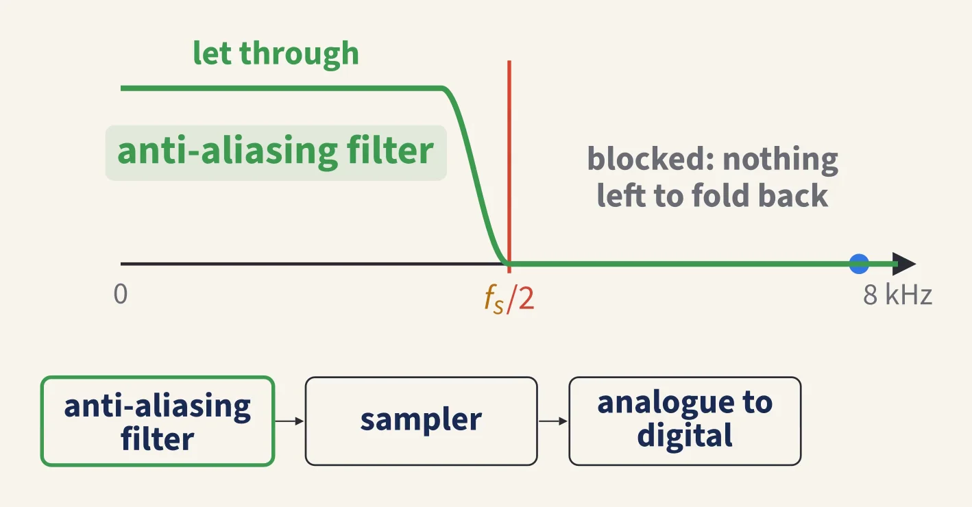
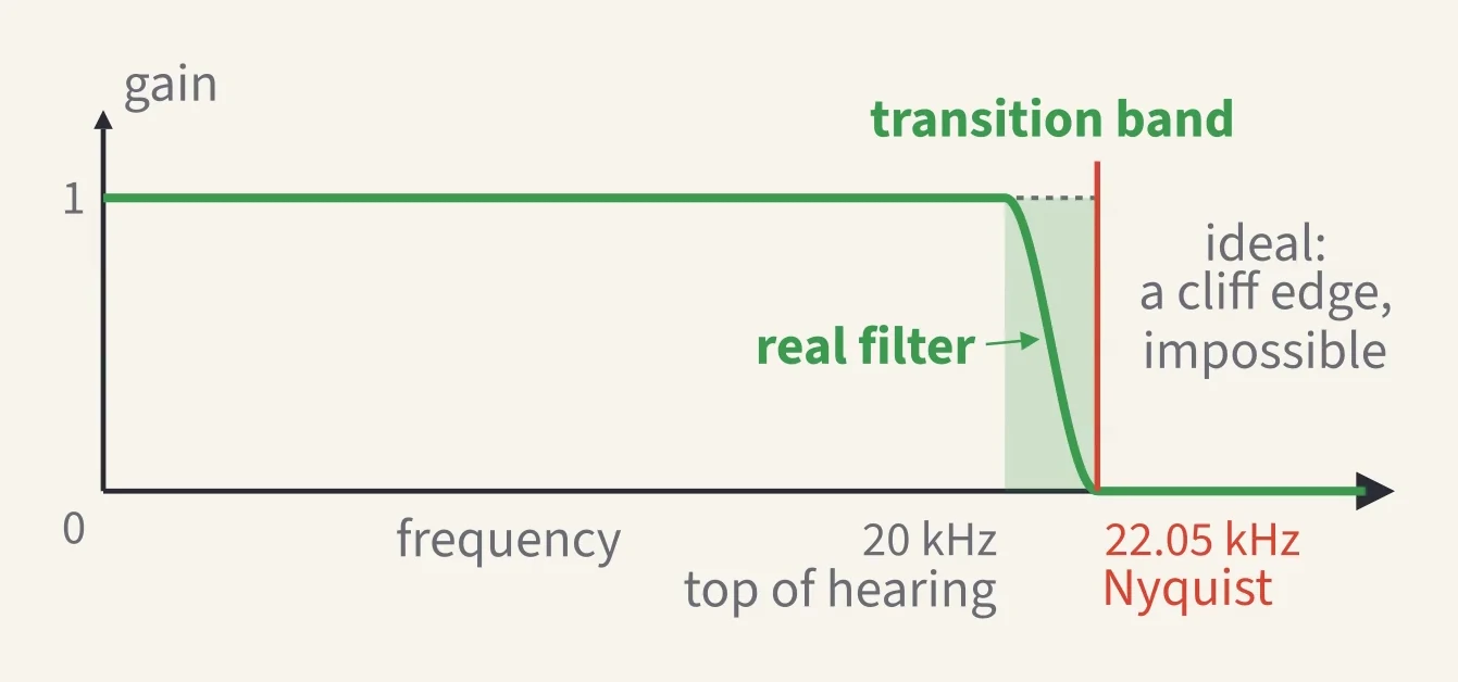
Once aliasing has happened, it cannot be undone from the samples alone. The alias sits among the real sound, and nothing done afterwards can tell them apart. So the only cure is prevention: before a signal is sampled, it passes through a low-pass filter that removes everything above the Nyquist frequency (a real filter cuts it down until any alias is too quiet to matter). This is the anti-aliasing filter, the first block of an analogue-to-digital system.
A real filter cannot cut off like a cliff edge. It needs a range of frequencies, its transition band, to go from letting sound through to blocking it. On a CD that range is the gap between 20 kHz, the top of hearing, and 22.05 kHz, the Nyquist frequency. That is what the spare room above 20 kHz is for.
That is the safe, simple rule. Strictly, the filter can keep falling until 24.1 kHz, because anything between 22.05 and 24.1 kHz folds back to somewhere above 20 kHz, out of the band we hear; the first-year part shows why. Real converters use that extra room.
The PCM transmitterin the video at 13:29
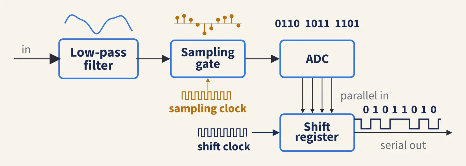
In Eduqas (WJEC) A Level Electronics this is the transmitter of a pulse code modulation (PCM) system. Its blocks, in order:
- Low-pass filter: removes frequencies above so they cannot alias.
- Sampling gate, driven by the sampling clock: takes a sample at each clock pulse.
- Analogue-to-digital converter (ADC): turns each sample into a binary number.
- Parallel-in serial-out (PISO) shift register, with its own clock: sends the number's bits out one at a time.
The low-pass filter comes first for exactly the reason above. The receiver mirrors the transmitter: a Schmitt trigger, a serial-in parallel-out (SIPO) shift register with its clock, a digital-to-analogue converter (DAC), and a second low-pass filter that smooths the output.
Part two · First-year university
Notes: the mathematics of aliasing and reconstruction
Frequencies that give the same samplesin the video at 16:23
Write a continuous tone as and keep it only at the sample times , where the integer (…, −1, 0, 1, 2, …) counts the samples. Since , the samples are
The samples depend only on the ratio , the frequency measured in cycles per sample. Now replace with . The ratio gains 1, so the angle gains : a whole number of complete turns, which changes nothing. So , , , and for any integer (positive, negative or zero), all give identical samples.
Cosine is an even function, , so a tone at gives the same samples as a tone at with its phase reversed ( becomes ). Put the two facts together and matches as well, again with its phase reversed: the mirror at the Nyquist frequency. For a cosine with zero phase the samples are identical; for a sine they come out upside down.
Finding any aliasin the video at 18:37
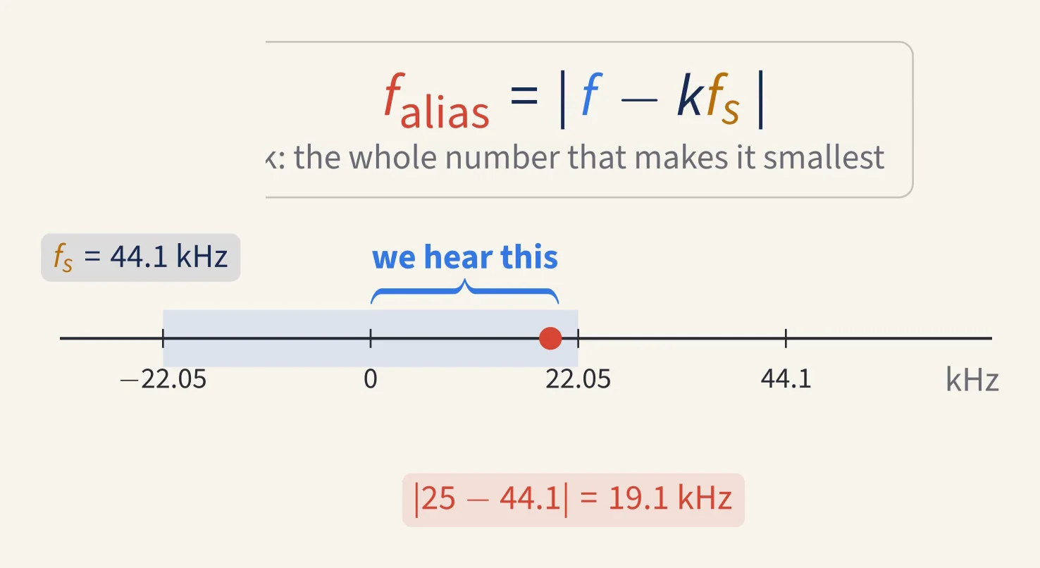
To find the alias of any frequency, shift it by whole multiples of until it lands between and , then take its size:
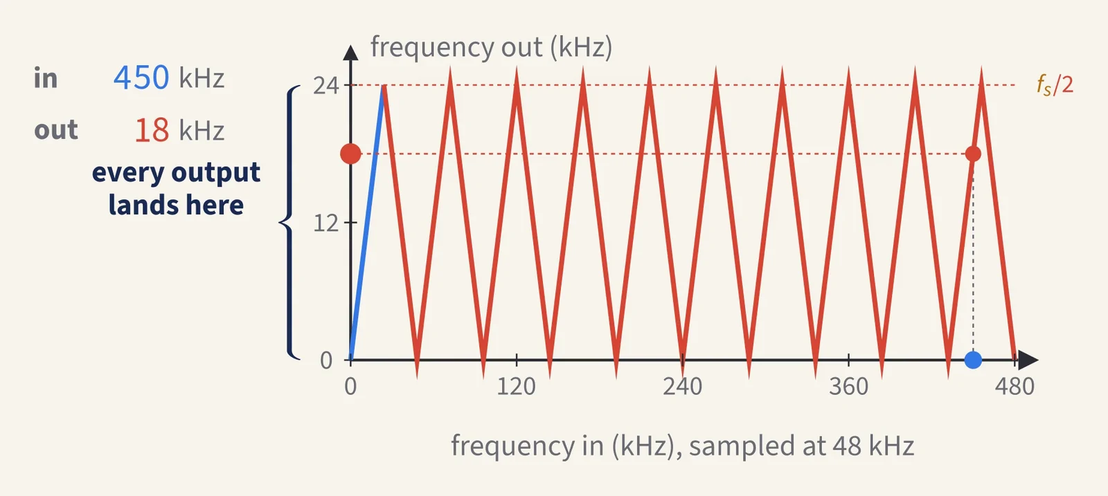
At kHz, 30 kHz gives kHz, 50 kHz gives 2 kHz, and 47 kHz gives 1 kHz. A tone at exactly 24 kHz, the Nyquist frequency, maps to itself, but it is the edge case where the samples can vanish.
Drawn as the frequency that comes out against the frequency that goes in, the rule is a straight line up to , then a zigzag: down to zero at , up to again at , and so on. Every input frequency, however high, lands somewhere between 0 and .
How steep the filter must be, and oversamplingin the video at 20:36
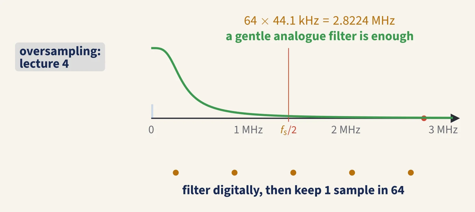
At 44.1 kHz anything above 22.05 kHz folds back, and the fold reaches down into the band we hear: 24.1 kHz lands exactly on 20 kHz. So the anti-aliasing filter must pass everything up to 20 kHz untouched and all but silence everything above 24.1 kHz. That is a very steep filter.
Modern converters avoid building it in analogue by oversampling. They sample far faster, often 64 times faster, so that a gentle analogue filter is enough; then they filter digitally and keep one sample in every 64. Lecture 4 shows how.
Getting the wave backin the video at 21:32
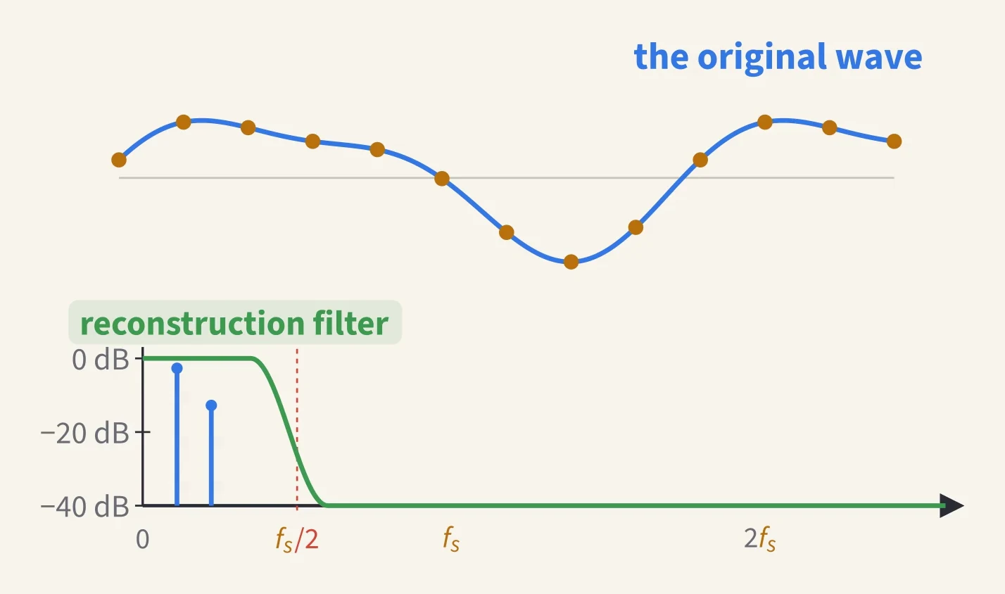
A digital-to-analogue converter can first produce a staircase, holding each sample's value until the next one arrives. The sharp edges of those steps are made of frequencies above the Nyquist frequency: copies of the signal, called images, around , and so on. A low-pass filter after the converter, the reconstruction or anti-imaging filter, removes them. Holding each value also tilts the top of the band down a little, by about 3 dB at 20 kHz for a CD, so real converters correct for that in the filter or oversample until the tilt is negligible. Provided the original held nothing at or above the Nyquist frequency, what is left is then not an approximation of the original wave: in the ideal case it is the original wave, slightly delayed and apart from the rounding of each sample, which is Lecture 2's subject.
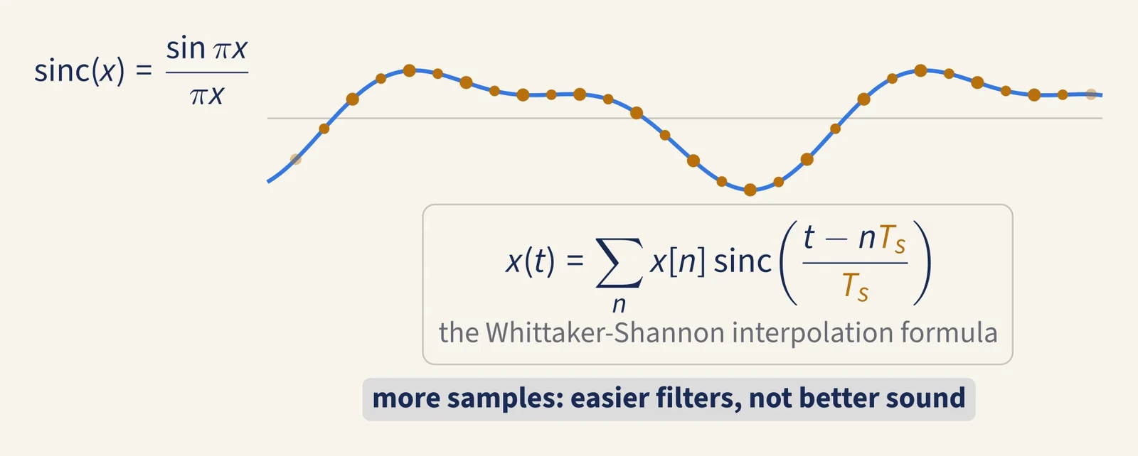
To see why, give every sample a bump shaped like the sinc function,
which is 1 at its own sample time and exactly 0 at every other sample time. Scale each bump by its sample's value and add them all up:
The sum passes through every sample and wiggles no faster than the Nyquist frequency allows. This is the Whittaker–Shannon interpolation formula, and in theory it rebuilds a band-limited signal exactly from its samples, using every sample, past and future. Real filters approximate it.
So digital audio is not steppy: below the Nyquist frequency, ideal sampling loses nothing. It also explains why more samples are not automatically better. Once the sampling rate is safely above twice the highest frequency you care about, extra samples make the filters easier to build, rather than the sound itself better.
Worked examples from the video
Every question the professor asks, with the moment it comes in the video. Try each one first, then open the working.
What is the period of a 440 Hz note (concert A)?
Show the working
s ms. Check the size: 440 cycles a second is a little under 500, so each cycle lasts a little over s ms.
How many samples per cycle does a 1 kHz tone get when sampled at 44.1 kHz?
Show the working
Samples per cycle, on average .
How many samples per cycle does a 20 kHz tone get at 44.1 kHz?
Show the working
samples per cycle on average: only just above two, the limit the sampling theorem sets.
What is the lowest sampling rate that can capture a bat's call reaching 100 kHz?
Show the working
kHz, so the sampling rate must be more than 200 kHz. 200 kHz itself, twice the highest frequency, is the boundary: sampled at exactly 200 kHz, a 100 kHz tone can vanish.
At a 48 kHz sampling rate, what do 30 kHz, 50 kHz and 47 kHz tones alias to?
Show the working
The Nyquist frequency is 24 kHz, so all three fold. With : kHz, kHz and kHz.
At 44.1 kHz, what does a 25 kHz tone alias to?
Show the working
25 kHz is above the Nyquist frequency of 22.05 kHz. With : kHz, inside the audio band, 0 to 20 kHz.
A signal contains frequencies up to 12 kHz. What is the minimum sampling rate?
Show the working
kHz, so the sampling rate must be more than 24 kHz. 24 kHz itself, twice the highest frequency, is the boundary: sampled at exactly 24 kHz, a 12 kHz tone can vanish.
A system samples at 32 kHz. What is its Nyquist frequency, and could it capture an 18 kHz tone?
Show the working
Nyquist frequency kHz. 18 kHz is above it, so no. Without an anti-aliasing filter it would alias to kHz; with the filter, it is cut down before sampling until that alias is too quiet to matter.
In a pulse code modulation transmitter, why must the low-pass filter come before the sampling gate, and not after it?
Show the working
Sampling is what creates the aliases. Once a frequency above has been sampled, its alias cannot be separated from the real signal, so a filter after the sampling gate would be too late. Frequencies above must be removed before sampling.
Practice set
Not in the video. Try each question before opening its answer. The same questions, with space to work and the answers at the back, are in the workbook.
A Level
A tone has a period of 0.5 ms. What is its frequency?
Answer
Hz kHz.
A system samples at 48 kHz. What is its sampling period?
Answer
.
A signal contains frequencies up to 15 kHz. What condition must the sampling rate satisfy?
Answer
kHz: more than 30 kHz. 30 kHz itself, the boundary, is not enough.
On average, how many samples does each cycle of a 5 kHz tone get at 44.1 kHz?
Answer
samples per cycle, on average.
A system samples at 22.05 kHz. What is its Nyquist frequency, and can it capture a 12 kHz tone?
Answer
Nyquist frequency kHz. 12 kHz is above it, so no. Without an anti-aliasing filter it would appear as an alias at kHz.
List the blocks of a PCM transmitter in order and say what each does.
Answer
Low-pass filter: removes frequencies above so they cannot alias. Sampling gate with sampling clock: takes a sample at each clock pulse. ADC: turns each sample into a binary number. PISO shift register with its clock: sends the number's bits out one at a time.
Explain why a filmed wheel can appear to turn slowly backwards.
Answer
A film camera usually samples 24 times a second. If a spoke moves just under one spoke-spacing between frames, the nearest match from one frame to the next is a small step backwards, so the fast forward motion looks like a slow backward one: aliasing in time.
First-year university
At kHz, find the alias of 40 kHz, 70 kHz and 100 kHz.
Answer
40: kHz. 70: gives kHz ( gives 26, larger). 100: gives kHz.
Show that gives the same samples as . What changes if the tone has a phase ?
Answer
, since adding changes nothing for an integer ; and , so it equals . With a phase, : the samples of a tone at with its phase reversed. So a sine at gives the samples of a sine at turned upside down.
Write the first four samples of at kHz. Which other frequency below 8 kHz gives the same samples?
Answer
The angles give . The same samples come from 5 kHz (): its angles give .
At kHz, which input frequencies alias into the audio band, 0 to 20 kHz, with (the copies around )?
Answer
Those within 20 kHz of : gives 24.1 kHz to 64.1 kHz. This is why the anti-aliasing filter must be deep by 24.1 kHz.
A sigma-delta converter oversamples 64 times a 44.1 kHz rate. What are its sampling rate and Nyquist frequency, and why does that help?
Answer
kHz MHz; its Nyquist frequency is 1.4112 MHz. Aliases now come only from far above the audio band, so a gentle analogue filter is enough; the steep filtering is done digitally before the rate is reduced.
Why does a zero-order-hold (staircase) DAC output contain frequencies above , and what removes them?
Answer
Each step's sudden jump needs high frequencies to form; in the spectrum they appear as images of the signal around , and so on. The reconstruction (anti-imaging) low-pass filter after the DAC removes them. Holding each value also droops the top of the band: the hold's response is , about dB at 20 kHz for a CD. So the filter also corrects that droop, or the converter oversamples until it is negligible; what is left is then the band-limited original.
Common misconceptions
“Digital audio comes out as a staircase.”
A DAC may produce steps first, but the reconstruction filter removes them and corrects the slight droop they cause. What comes out is, ideally, the original band-limited wave, rebuilt from the samples. More in the notes
“More samples always sound better.”
Once the sampling rate is more than twice the highest frequency present, the samples already hold the whole signal. A higher rate mainly makes the filters easier to build. More in the notes
“Frequencies above the Nyquist frequency just disappear.”
They fold back as aliases at lower frequencies, and after sampling nothing can tell them apart from real tones. That is why the filter comes before the sampler. More in the notes
“Exactly two samples per cycle is enough.”
At exactly two the samples can land on the zero crossings and the wave vanishes. The sampling rate must be more than twice the highest frequency. More in the notes
Terms in this lecture
- signal
- amplitude
- period
- frequency
- phase
- analogue signal
- digital signal
- quantisation
- sampling
- sampling rate
- sampling period
- sampling theorem
- Nyquist frequency
- aliasing
- anti-aliasing filter
- transition band
- pulse code modulation
- analogue-to-digital converter
- digital-to-analogue converter
- oversampling
- reconstruction filter
- image
- sinc function
- Whittaker–Shannon interpolation formula
Exam specifications this lecture teaches
Checked against each board's own specification on 28 October 2026. Spec points are summarised in our words; the page number leads to the exact wording. No board has endorsed this site.
| Qualification | Spec point | Coverage | Where in this lecture |
|---|---|---|---|
| Eduqas A Level Electronics | Component 2, topic 4 (d) the sampling frequency needed for a given highest signal frequency; the Nyquist theorem (A level only; page 33 (31)) | covered | The sampling theorem, Why a CD samples at 44.1 kHz |
| OCR A Level Physics B (Advancing Physics) | 3.1.1 (c)(vii) a minimum sampling rate of more than twice the highest frequency (AS; page 23 (16)) | covered | The sampling theorem |
| Pearson Edexcel A level Music Technology | Component 3, AoS 3, 3.1 (bullet: sampling theory and converters) digital hardware: sampling theory and converters (not stated; page 44 (40)) | covered | Sampling, The sampling theorem, The anti-aliasing filter |
| Eduqas A Level Electronics | Component 2, topic 4 (c) the PCM link as a block diagram: the transmitter (low-pass filter, sampling gate and clock, ADC, PISO register) and the receiver (Schmitt trigger, SIPO register, DAC, low-pass filter) (A level only; page 33 (31)) | partly covered Lecture 1 explains and diagrams the transmitter; the receiver is only listed. | The PCM transmitter, The anti-aliasing filter, Getting the wave back |
| Eduqas A Level Electronics | Component 1, topic 4 (e) digitising audio; the effect of sampling rate and resolution (A level only; page 21 (19)) | partly covered Lecture 1 covers the sampling rate; resolution is Lecture 2. | Why go digital?, Sampling |
| AQA A-level Computer Science | 3.5.6.5 (AS) and 4.5.6.7 digital representation of sound: sample resolution, sampling rate, the Nyquist theorem; sample size in bytes (AS and A-level; page 27 and 71) | partly covered Lecture 1 covers the sampling rate and the Nyquist theorem; sample resolution is Lecture 2. | Sampling, The sampling theorem |
| OCR A Level Physics B (Advancing Physics) | 3.1.1 (a)(iii) digitising a signal, which may contain noise; the advantages and disadvantages of digital signals (AS; page 22 (15)) | partly covered Lecture 1 gives the advantages of digital signals; it does not cover noise in the signal or the disadvantages. | Why go digital? |
| AQA A-level Physics | 3.13.2.1 (Electronics option) sampling audio for digital transmission: sampling rate, quantisation, the pros and cons of digital sampling, recovering data from noise, PCM (A-level only, option; page 64) | partly covered Lecture 1 covers sampling and PCM; quantisation is Lecture 2. | Why go digital?, Sampling, The PCM transmitter |
| Pearson Edexcel A level Music Technology | Component 4, AoS 2, 2.4 specifications of digital recordings: A/D and D/A conversion, sample rate, bit depth, uncompressed PCM (not stated; page 54 (50)) | partly covered Lecture 1 covers sample rate and conversion; bit depth is Lecture 2. | Sampling, Why a CD samples at 44.1 kHz, Getting the wave back |
| Pearson Edexcel A level Music Technology | Component 4, AoS 2, 2.5 (bullet: calculations describing sound waves) calculations describing sound waves: frequency, phase, amplitude (not stated; page 54 (50)) | partly covered Lecture 1 calculates frequency and period; phase and amplitude are described but not calculated. | What a signal is |
| OCR A Level Physics B (Advancing Physics) | 3.1.1 (c)(viii) data rate = samples per second × bits per sample (AS; page 23 (16)) | background Lecture 1 defines the sampling rate, one factor in this calculation; it does not teach the data-rate equation. | Sampling |
| AQA A-level Physics | 3.3.1.1 amplitude, frequency, wavelength, phase; f = 1/T (AS; page 18) | background | What a signal is |
| Eduqas A Level Physics | Component 3, topic 1 (e) displacement, amplitude, wavelength, frequency, period (not stated; page 39 (36)) | background | What a signal is |
| Qualifications Scotland (formerly SQA) Advanced Higher Physics | Quanta and waves: Waves the travelling-wave equation with amplitude, frequency and phase (Advanced Higher; page 17 (15)) | background | What a signal is |
References
Read next
- Richard G. Lyons, Understanding Digital Signal Processing, 3rd edition, Pearson, 2011. Chapter 2, "Periodic Sampling". The friendliest next step after this lecture: aliasing and sampling, with plenty of pictures. Checked 28 October 2026.
- Steven W. Smith, The Scientist and Engineer's Guide to Digital Signal Processing, 1997. Chapter 3, "ADC and DAC". Free online and readable at A level. It uses "Nyquist frequency" and "Nyquist rate" for the same thing, and says why the terms get muddled. Checked 28 October 2026.
- Alan V. Oppenheim and Ronald W. Schafer, Discrete-Time Signal Processing, 3rd edition, 2010. Chapter 4, "Sampling of Continuous-Time Signals", pp. 153–273. The standard university text, now free on MIT OpenCourseWare. Section 4.3 is the sinc rebuild; 4.8 and 4.9 are the anti-aliasing filter, the DAC and oversampling. Checked 28 October 2026.
- Ken C. Pohlmann, Principles of Digital Audio, 6th edition, McGraw Hill, 2011. Chapter 2, "Fundamentals of Digital Audio". The audio engineer's book: chapters on the compact disc and on sigma-delta converters, and an appendix on the sampling theorem. Checked 28 October 2026.
The original papers
- E. T. Whittaker, "On the Functions which are represented by the Expansions of the Interpolation-Theory", Proceedings of the Royal Society of Edinburgh 35, 181–194 (1915). An early, influential development of the interpolation formula behind the sinc rebuild. Checked 28 October 2026.
- H. Nyquist, "Certain Topics in Telegraph Transmission Theory", Transactions of the AIEE 47(2), 617–644 (1928). The telegraph paper behind the factor of two and the name. Not free to read; reprinted in Proc. IEEE 90(2), 2002. Checked 28 October 2026.
- V. A. Kotelnikov, "On the transmission capacity of 'ether' and wire in electric communications" (1933), English translation in Physics-Uspekhi 49(7), 736–744 (2006). The theorem stated for communications engineers, in Russian, in 1933. The publisher lets teachers and students read the translation free. Checked 28 October 2026.
- C. E. Shannon, "Communication in the Presence of Noise", Proceedings of the IRE 37(1), 10–21 (1949). The paper that made the theorem famous. Not free to read; reprinted in Proc. IEEE 86(2), 1998. Checked 28 October 2026.
The standard
- IEC 60908:1999, Audio recording: Compact disc digital audio system, edition 2.0. The compact disc standard, still the current edition. Sold by the IEC. Checked 28 October 2026.
Where the facts in these notes come from
- NPL, Kaye & Laby Tables of Physical and Chemical Constants, 2.4.1 "The speed and attenuation of sound" (archived copy). 343.5 to 344.5 m/s in air at 20 °C, for humidity between 10% and 90%. The film rounds it to about 340. Checked 28 October 2026.
- D. Purves and others (eds), Neuroscience, 2nd edition, Sinauer, 2001, "The Audible Spectrum". Hearing from about 20 Hz to 20 kHz, and a lower top end in most adults. Free on the NCBI Bookshelf. Checked 28 October 2026.
- K. A. Schouhamer Immink, "The CD Story", Journal of the AES 46, 458–465 (1998). A member of the Philips CD team on how the CD's numbers were chosen, 44.1 kHz among them. Free on the author's site. Checked 28 October 2026.
- E. Meijering, "A chronology of interpolation: from ancient astronomy to modern signal and image processing", Proceedings of the IEEE 90(3), 319–342 (2002). Who found the sampling theorem, and when: Whittaker, Nyquist, Kotelnikov, Shannon and others, each in their own field. Free copy at EPFL. Checked 28 October 2026.
- Digital Cinema Initiatives, Digital Cinema System Specification, version 1.5.1, section 3.1.4.2 "Frame Rates". Digital cinema masters must support 24 frames a second, the usual rate for films. Checked 28 October 2026.
- Texas Instruments, PCM1808 Single-Ended, Analog-Input 24-Bit, 96-kHz Stereo ADC, datasheet SLES177B. A real audio converter that samples 64 times faster than its output rate, as in the oversampling section. Checked 28 October 2026.
Where the field is now
Beyond the exam: recent work for the curious, each summarised at this lecture's level and checked against the paper itself.
A Meta-Analysis of High Resolution Audio Perceptual Evaluation
Joshua D. Reiss, Journal of the Audio Engineering Society 64(6), 364–379 (2016) · Peer-reviewed meta-analysis, 2016 · Free to read · checked 28 October 2026
Can listeners tell standard audio (16 bits, 44.1 or 48 kHz) from "high-resolution" audio with higher sampling rates or more bits? Pooling 18 listening experiments with more than 400 listeners, this study finds a small but statistically significant ability to tell them apart, much stronger after training. Why is still unknown, and the result does not show that people hear tones above 20 kHz.
Extended high frequency hearing and speech perception implications in adults and children
Lisa L. Hunter and others, Hearing Research 397, 107922 (2020) · Peer-reviewed review, 2020 · Free (PubMed Central) · checked 28 October 2026
Standard hearing tests stop at 8 kHz, though young ears hear up to about 20 kHz. This review finds that the range above 8 kHz helps us follow speech in noise, and is the first to go with age, loud noise, ear infections and some medicines. It can be measured reliably and may give early warning of hearing loss; whether losing it causes trouble with speech in noise is still open.
Compressed sensing MRI: a review from signal processing perspective
Jong Chul Ye, BMC Biomedical Engineering 1, 8 (2019) · Peer-reviewed review, 2019 · Open access (CC BY 4.0) · checked 28 October 2026
An MRI scanner samples the spatial frequencies of the body, and taking enough samples to meet the Nyquist criterion makes scans slow. Compressed sensing rebuilds an accurate image from far fewer samples by using extra knowledge: the image can be described by few numbers once transformed (it is sparse in wavelets, for example), and the samples are chosen to suit. So it does not break the sampling theorem. It is now approved in commercial scanners; computing cost and quality at high speed-ups remain problems, and the author points to fast progress in deep-learning reconstruction, which is closely related.
An Overview of Noise-Shaping SAR ADC: From Fundamentals to the Frontier
Lu Jie and others, IEEE Open Journal of the Solid-State Circuits Society 1, 149–161 (2021) · Peer-reviewed review, 2021; technical · Open access (CC BY 4.0) · checked 28 October 2026
For students who liked the oversampling section. Noise-shaping SAR converters, which appeared in the 2010s, join the low-power successive-approximation converter to the noise shaping of sigma-delta converters (Lecture 4). The paper explains how they work and what limits them. Across chips published to mid-2021, their efficiency figure improves by about 6.4 dB per decade; the chip-making process matters a lot, though the best results so far come from mid-range 28 to 65 nm processes rather than the newest.
How this page was checked
Checked by two AI reviewers against cited sources, 28 October 2026.Lecturer review pending.
| Check | Result | Date |
|---|---|---|
| Claude (Anthropic), in a fresh context, independently, against the cited sources | 25 findings, 25 settled. Two errors in the first-year maths (a staircase DAC's droop, and the phase of a mirrored frequency), both fixed; the rest were wording, exam-spec coverage, research summaries and alt text, all corrected. | 28 October 2026 |
| ChatGPT (OpenAI), through Codex, independently, against the cited sources | 37 findings, 37 settled. 31 on its first read, including the same two errors, and 6 more when it then checked every fix; all corrected. | 28 October 2026 |
| Every numerical answer recomputed by code | All match | every build |
| University lecturer | Pending | – |
Found a mistake? Tell us, and it will be checked and corrected here with a note of what changed. How we check every page.